This release note accompanies the R code used in the Practical session #2 - Mapping deep-water fishing grounds: from fishing tracks to fishing effort maps. It aims to detail part of the workflow adopted to elaborate Automatic Identification System (AIS) data in the context of the GFCM initiative to map fishing grounds for deep-water red shrimp in the Eastern-Central Mediterranean Sea. The processing workflow (Figure 1) is divided into three scripts and serve to (i) pre-process fishing tracks and to aggregate data for different purposes: (ii) fishing effort patterns and (iii) fishing pressure indicators. Results of points (ii) and (iii) are both visualized as map and as monthly time-series. Each step is shown as code chunk and it is briefly described.

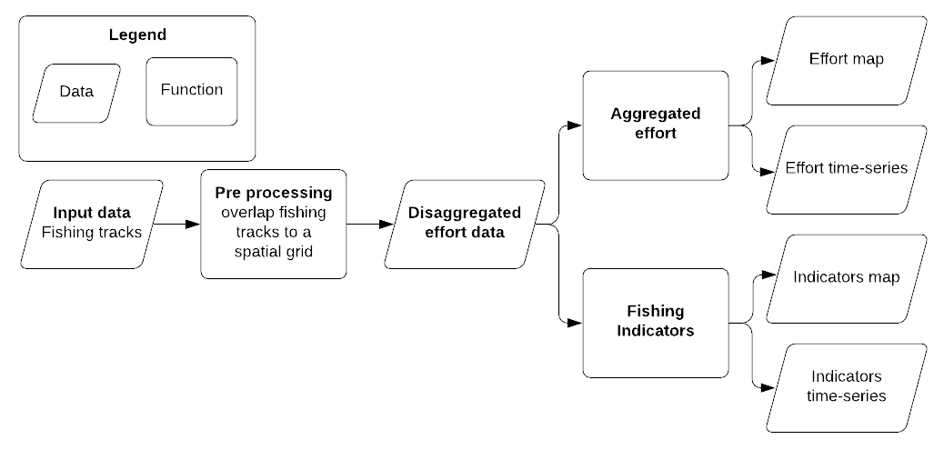
Figure 1: Conceptual workflow used in the Practical session #2 - Mapping deep-water fishing grounds: from fishing tracks to fishing effort maps

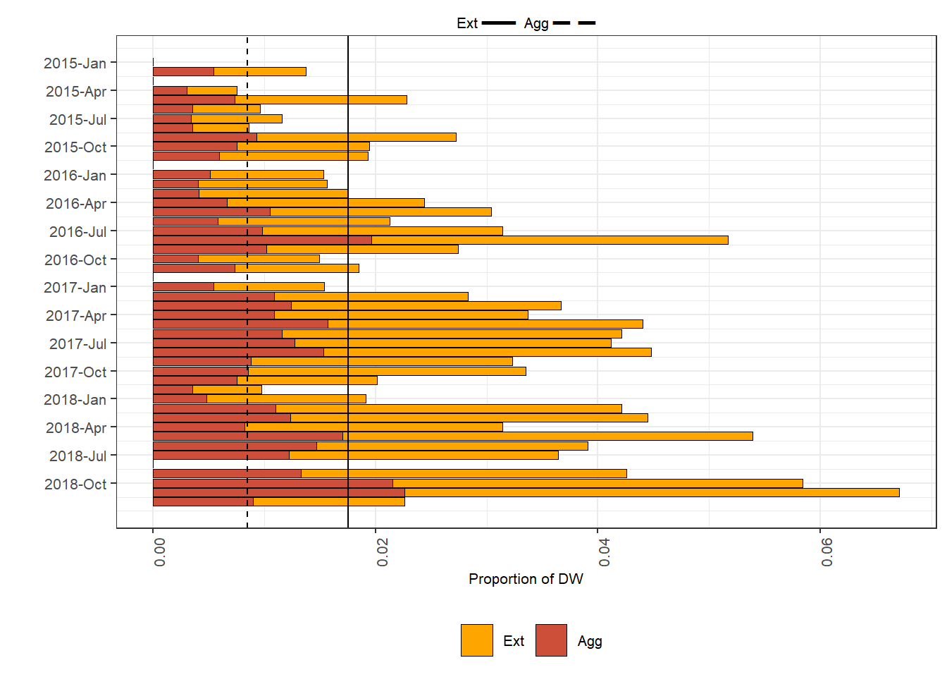
The results are some of the plots shown in the chapter 3.4 of the DWRS report on the fishing ground mapping (not yet published), in particular those referring to the aggregated fishing effort (Figure 2 a and b) and to the indicators of fishing pressure (Figure 2 c and d).

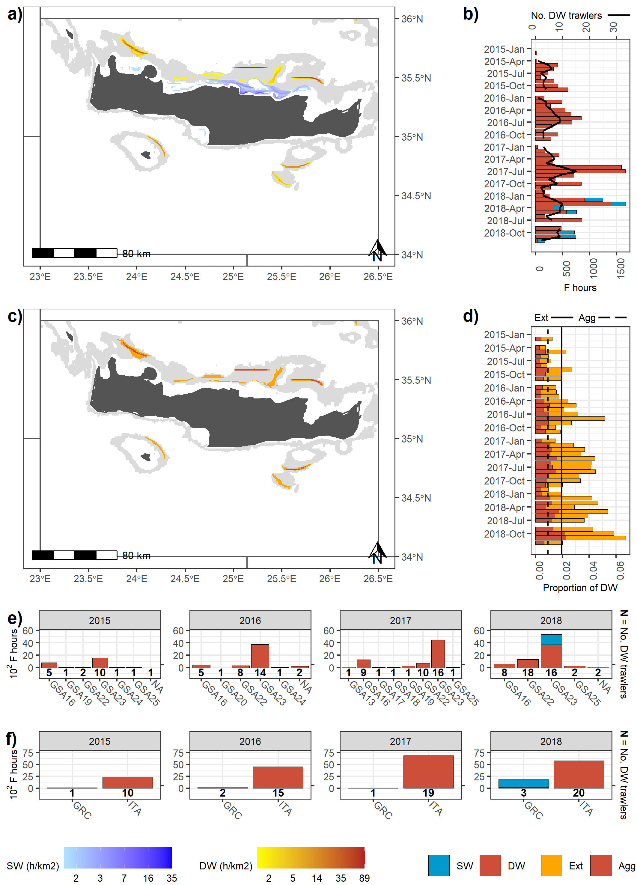
Figure 2: Fishing activities of vessels DW trawling in GSA 23. (a) Spatial distribution of mean DW and SW fishing activities during the study period; (b) Monthly fishing hours in DW (red) and SW (blue), and number of DW trawlers exerting these activities (solid line); (c) Spatial distribution of fishing pressure indicators of Extension (orange) and Aggregation (red) during the study period; (d) Monthly proportions of the DW area trawled and average values for fishing pressure indicators of extension (orange bars and solid line, respectively) and aggregation (red bars and dashed line, respectively); (e - f) Annual fishing hours in DW (red) and SW (blue) by GSA of arrival and country, and number of DW trawlers exerting these activities

Input data

Input data required to start the workflow are described below

Fishing data

The fishing data are loaded as f_tracks in the first script (see below) and are here briefly introduced:

MMSI	year	month	gear	trip	id_track	s_time	f_time	range	geometry
1	2015	2	OTB	126	85	2015-02-09 08:58:42	2015-02-09 10:43:52	NA	LINESTRING (24.6528 35.0631…
1	2015	2	OTB	126	86	2015-02-09 11:13:55	2015-02-09 13:19:10	NA	LINESTRING (24.702 35.0109,…
1	2015	2	OTB	127	87	2015-02-11 09:07:40	2015-02-11 09:42:43	NA	LINESTRING (24.6769 35.0626…
1	2015	2	OTB	127	88	2015-02-11 10:22:46	2015-02-11 13:53:04	NA	LINESTRING (24.711 35.0207,…
1	2015	2	OTB	127	89	2015-02-11 14:23:07	2015-02-11 14:43:07	NA	LINESTRING (24.7117 35.0399…
1	2015	2	OTB	127	90	2015-02-11 15:28:10	2015-02-11 16:39:43	NA	LINESTRING (24.704 35.0097,…

Where:

MMSI: identifier of the vessel responsible for the fishing activity. Dummy data provided for privacy purposes.
year: year in which the fishing activity was observed
month: month in which the fishing activity was observed
gear: gear predicted for the fishing activity
trip: identifier of the trip where the fishing activity was observed
id_track: identifier of the fishing track
s_time: start time of the fishing track
f_time: end time of the fishing track
range: parameter that applies to Purse Seine fishing activity
geometry: spatial attribute

Fishing data provided are distributed as in the map here shown:

Spatial layers

Fours vector layers are required to perform the functions foreseen by the workflow:

grid: a 1km by 1km grid covering the GSA 23, with additional attributes indicating the bottom type and if the cell is or not within the 400-800 m bathymetry.
land: contour of land
gsa: boundaries of the GFCM-GSA
dep: contour of the 400-800m batymetry

grid <- read_sf("maps/grid")

land=read_sf("maps/land")%>% 
  st_crop(., xmin=-10, xmax=43, ymin=20, ymax=48) #

gsa<-read_sf("maps/gsa")%>%
  dplyr::filter(SMU_CODE == '23' )

dep = read_sf("maps/depth_contours")%>%
  st_cast(., to = "POLYGON")%>%
  st_set_crs(st_crs(gsa))%>%
  st_buffer(0)%>%
  st_crop(gsa)

lims=c(st_bbox(gsa[c(1,3)], st_bbox(gsa[c(2,4)])))

Processing

The proposed workflow is hereafter applied on the fishing tracks of a single area although it can be iterated on multiple areas. It is organized into three scripts:

PreProcessing: it aims to overlap fishing tracks to a spatial grid.
FishingPattern: it starts from the output of the first script and it aggregate data to produce and visualize fishing effort pattern
FishingIndicators: it starts from the output of the first script and it aggregate data to produce and visualize fishing effort indicators

Pre processing

The topic of this first section is the overlap of the fishing track to a grid covering the reference area. This is a key-step and its output will represent the basis for all the images contained in the Figure 2.

Before to start

Check the working directory (WD), which have to be “practical_session_2”. The getwd() command shows you which is your WD. If you just opened the project, push on the setwd('practical_session_2/') line. In case you need to go back of one folder, the setwd('..') command sets the WD to a backward place.

Load spatial Data and set parameters

The first part of the code aims to prepare the environment for the processing of the fishing data. Loading the spatial grid:

grid=read_sf("maps/grid")

Defining two parameters:

activate_filter activates a filter to the data to remove outliers (see below in Step 4)
ref_years indicate the time span of the analysis

activate_filter='Y'
ref_years=2015:2018

For loop sectioned

In the original code, all the following steps are done within a for loop iterating on the years (as defined by ref_years). For illustrative purposes, here we present all the operations outside the for loop, taking the year 2015 as example.

Step 1

Load the fishing data for one year (2015 used as example)

f_tracks=read_sf(file.path("data",2015,paste0("f_segments_DWRS_WS_", 2015, ".shp")))
f_tracks$s_time=as_datetime(f_tracks$s_time, tz='UTC')
f_tracks$f_time=as_datetime(f_tracks$f_time, tz='UTC')

Step 2

The next step deals with applying the estimate_fishing_effort_DWRS function on the data for each vessel. This function, which is inherited from the R4ais workflow, is defined in a separate script. Here below is shown the original code. The function performs a spatial intersection between the fishing tracks and the grid cells, then it aggregates the results to obtain the fishing activity occurring within each grid cell. The difference with the R4ais version is in the factors used to aggregate the data: data are aggregated by the factors grid_id+gear+MMSI+trip+s_time, while in the R4ais only by grid_id+gear. This modification was needed to keep data at the maximum level of disaggregation, permitting later to use the same dataset for multiple purposes.

estimate_fishing_effort_DWRS <- function(fishing_tracks, grid){
  lapply(fishing_tracks, function(x){
    if(is.data.frame(x)){
      x = st_sf(x)
    }
    xgear = unique(x$gear)
    st_crs(x)=wgs # set crs 
    if(xgear == "PS"){
      x$duration=difftime(x$f_time, x$s_time, units="secs")
      x=st_as_sf(x)
      xint=st_intersection(grid, x)
      xint=data.frame(xint)
      xint=xint[,c("grid_id", "gear", "duration")]
      xint$fishing_hours=xint$duration/3600
      f_hours = aggregate(fishing_hours~grid_id+gear, data = xint, sum)
      colnames(f_hours)[ncol(f_hours)] = "f_hours"
      grid_edit=merge(grid, f_hours, by="grid_id") # combine effort to grid
      return(grid_edit)
    }else{
      xnames=names(x)
      x$distance=st_length(x$geometry, units="m") # estimated fishing track 
      x$duration=difftime(x$f_time, x$s_time, units="secs")
      x$speed_ms=as.numeric(x$distance)/as.numeric(x$duration)
      x$speed_kn=x$speed_ms*1.94384
      x=st_as_sf(x)
      xint=st_intersection(grid, x)
      if(nrow(xint) > 0){
        xint$observed_swept=st_length(xint)
        xint=data.frame(xint)
        xint=xint[,c("grid_id","MMSI", "trip", "s_time" ,"gear","observed_swept", "speed_ms")]
        xint$fishing_hours=(as.numeric(xint$observed_swept)/xint$speed_ms)/3600
        xint
        f_hours = aggregate(fishing_hours~grid_id+gear+MMSI+trip+s_time, data = xint, sum)  # estimate fishing effort in cells grid
        colnames(f_hours)[ncol(f_hours)] = "f_hours"
        grid_edit=merge(grid, f_hours, by="grid_id") # combine effort to grid
        grid_edit=grid_edit[grid_edit$f_hours>0,]
        grid_edit=grid_edit[,c("MMSI","gear", "trip", "s_time" , 'G_ID', 'DW', 'f_hours')]
        return(grid_edit)
      }
    }
  })
  
}

Data are first divided into a list by vessel identifier and then the estimate_fishing_effort_DWRS function is applied on each element of the list.

f_tracks=split(f_tracks, f_tracks$MMSI)
f_tracks_grid=estimate_fishing_effort_DWRS(f_tracks, grid)

Step 3

As the output of the estimate_fishing_effort_DWRS function is a list, the data need to be unlisted and formatted. Later on, the information regarding year and month of the fishing activity it is added.

  f_tracks_grid=plyr::ldply(f_tracks_grid,.id = NULL)
  f_tracks_grid=f_tracks_grid[ , -which(names(f_tracks_grid) %in% c("grid_id", 'geometry'))]  ## remove not useful information
  f_tracks_grid$month=lubridate::month(f_tracks_grid$s_time)
  f_tracks_grid$year=lubridate::year(f_tracks_grid$s_time)

Step 4 (Optional)

To remove some outliers, we may exclude grid cells where fishing activities over the entire year were fished for less than 0.33 hours.

 if(activate_filter=="Y"){
    print("Filtering activated")
    outlier_filter=aggregate(x=f_tracks_grid$f_hours, by=list('G_ID'=f_tracks_grid$G_ID,'year'=f_tracks_grid$year ), FUN=sum)
    outlier_filter=outlier_filter[outlier_filter$x>=0.33,c('G_ID','year')]
    f_tracks_grid=merge(outlier_filter, f_tracks_grid, by=c("G_ID", "year"), all.x=T)
  }

## [1] "Filtering activated"

Results

The resulting data fishing_data is the base grid having the cells filled with the information of fishing activity. Each row refers to the intersection between a grid cell G_ID and a unique fishing track defined by its starting time s_time and the fishing vessel MMSI performing it. Therefore each fishing track is divided into as many rows as the number of grid cells intersected. This type of information permits to aggregate the fishing activity in all the format needed for the further analysis.

Here it is shown the header of the dataset.

G_ID	year	MMSI	gear	trip	s_time	DW	f_hours	month
1872289	2015	1	OTB	149	2015-09-25 18:58:07	1	0.2296348	9
1872289	2015	1	OTB	151	2015-09-29 06:35:27	1	0.2491466	9
1872289	2015	1	OTB	149	2015-09-25 08:32:07	1	0.1997793	9
1872289	2015	1	OTB	150	2015-09-28 16:49:15	1	0.2390655	9
1872289	2015	1	OTB	149	2015-09-25 09:37:10	1	0.0942475	9
1872290	2015	1	OTB	150	2015-09-28 16:49:15	1	0.2367738	9

Where:

G_ID: id of the grid cell
year: year in which the fishing activity was observed
MMSI: identifier of the vessel responsible for the fishing activity
gear: gear predicted for the fishing activity
trip: identifier of the trip where the fishing activity was observed
s_time: start time of the fishing track (not related to the grid cell)
DW: binary column indicating if the grid cell falls in the DW stratum.
f_hours: fishing hours observed in the G_ID grid cell for the specific fishing track starting at s_time and performed by the MMSI vessel
month: month in which the fishing activity was observed

FishingPattern

This section presents the code used to produce the Figure 35.a of the DWS-Fishing activity report. It is a thematic map showing the mean fishing hours by grid cell in the GSA 23, over the period january 2015-december 2018.

Before to start

Load data

The input data is represented by the output of the PreProcessing.R script and by the spatial data introduced at the beginning of the lesson. In addition, it is loaded an R script containing the default setting for the base map used.

fishing_data= read_csv("data/fishing_data.csv")


rm(vessel_selection)
# Shapefiles 
grid <- read_sf("maps/grid")

land=read_sf("maps/land")%>% 
  st_crop(., xmin=-10, xmax=43, ymin=20, ymax=48)

gsa=read_sf("maps/gsa")%>%
  dplyr::filter(SMU_CODE == '23' )

dep = read_sf("maps/depth_contours")%>%
  st_cast(., to = "POLYGON")%>%
  st_set_crs(st_crs(gsa))%>%
  st_buffer(0)%>%
  st_crop(gsa)

lims=c(st_bbox(gsa[c(1,3)], st_bbox(gsa[c(2,4)])))

text_size=8
plot_height=25
plot_width=18
source("R/supporting_code/plot_specifications.R")

defo_map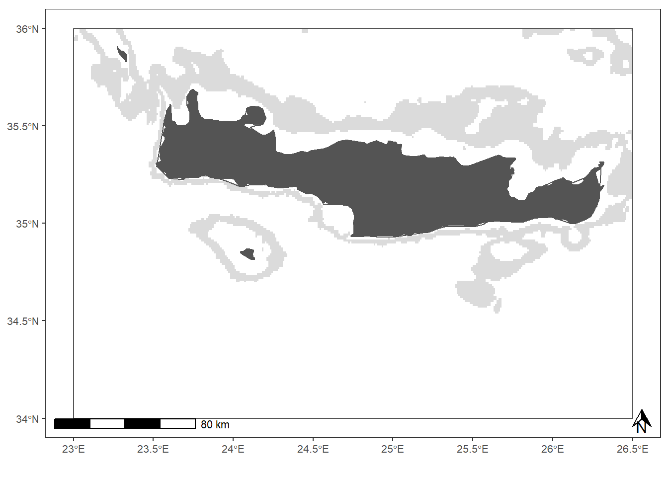

Optional

In the following line there is the possibility to reduce the dataset by selecting only those vessels that fished in the DW strata at least once in a month.

vessel_selection=unique(fishing_data[fishing_data$DW==1,c('MMSI','month','year')]) # Create a monthly list of vessels fishing in the DW strata

fishing_data=merge(vessel_selection, fishing_data, by=c("MMSI", "year", "month"), all.x = T)

Effort Map

Step 1

The fishing_data dataset is aggregated to get mean annual fishing intensity by grid cell. This is done in two consecutive aggregation functions. The cumulative_hours_by_year dataset is the annual cumulative values of fishing activity by grid cell. In the following line, the same dataset is further summarized into mean_hours_over_year, which is the mean value by cell over the years.

cumulative_hours_by_year=aggregate(list(f_hours_year=fishing_data$f_hours), 
                             by=list('G_ID'= fishing_data$G_ID ,'year'=fishing_data$year), FUN=sum)

mean_hours_over_year=aggregate(list(f_hours_overall=cumulative_hours_by_year$f_hours_year), 
                               by=list('G_ID'=cumulative_hours_by_year$G_ID),FUN=mean)

G_ID	f_hours_overall
1867864	0.5300249
1868595	0.3755053
1869328	0.4563027
1870067	0.4577012
1870808	1.2239307
1870810	0.4821836

Step 2

Now that the overall fishing intensity by grid cell is obtained, it is possible to paste this information to the base grid. This is done by using the merge function, using the G_ID column as primary key. An additional column with the log of fishing hours is also created

grid_fishing=merge(grid, mean_hours_over_year, by='G_ID', all.x=F)
grid_fishing$f_hours_log=log(grid_fishing$f_hours + 1)

G_ID	DW	GSA	EUNIScomb	grid_id	f_hours_overall	geometry	f_hours_log
1867864	1	GSA23	A6.511	15016	0.5300249	POLYGON ((23.79001 35.84624…	0.4252840
1868595	1	GSA23	A6.511	15186	0.3755053	POLYGON ((23.80001 35.84624…	0.3188211
1869328	1	GSA23	A6.511	15357	0.4563027	POLYGON ((23.81001 35.84624…	0.3759008
1870067	1	GSA23	A6.511	15529	0.4577012	POLYGON ((23.82001 35.83624…	0.3768607
1870808	1	GSA23	A6.511	15700	1.2239307	POLYGON ((23.83001 35.83624…	0.7992762
1870810	1	GSA23	A6.511	15702	0.4821836	POLYGON ((23.83001 35.81624…	0.3935164

This is how the grid populated with fishing activity appears. The interactive map is just for illustrative purposes and it is not part of the R code used for the course.

Step 3

To facilitate the plotting, grid data are divided by depth in two separate files (grid_DW and grid_SW). Fishing hours are also normalized.

grid_DW=grid_fishing[grid_fishing$DW==1,]
grid_DW$f_hours_log_st=st_fun(grid_DW$f_hours_log)

grid_SW=grid_fishing[grid_fishing$DW==0,]
grid_SW$f_hours_log_st=st_fun(grid_SW$f_hours_log)

Plot

Specifications for the plot

Plots are standardized between figures using the settings loaded at the beginning of the script. In addition, labeling can be optimized to fit the data of each area.

brks_DW = seq(0, 1, length.out = 10)[c(2,4,6,8,10)]
brks_DW_lab = round(exp((brks_DW*(max(grid_DW$f_hours_log) - min(grid_DW$f_hours_log))) + min(grid_DW$f_hours_log)))

brks_SW = seq(0, 1, length.out = 10)[c(2,4,6,8,10)]
brks_SW_lab = round(exp((brks_SW*(max(grid_SW$f_hours_log) - min(grid_SW$f_hours_log))) + min(grid_SW$f_hours_log)))

Result

The object defo_map contains all the settings specified above and represents the basis of our plot. Here are added the effort statistics, along with the parameters to set the legend values appropriately.

plot_effort_map = defo_map+
  geom_sf(data = grid_SW, aes(fill = f_hours_log_st), colour = NA, alpha = 0.8, show.legend = "point" ) +
  scale_fill_gradient(low = "lightskyblue1", high = "blue", breaks = brks_SW, labels = brks_SW_lab, guide = guide_colorbar(title = "SW (h/km2)")) +
  new_scale("fill") +  
  geom_sf(data = grid_DW, aes(fill = f_hours_log_st), colour = NA) +
  scale_fill_gradient("DW (h/km2)", breaks = brks_DW, labels = brks_DW_lab, low = "yellow", high = "firebrick") +
  coord_sf(xlim=c(lims[[1]], lims[[3]]), ylim=c(lims[[2]], lims[[4]]) , label_axes = list(bottom = "E", right = "N")) +
  xlab("") ; plot_effort_map

## Coordinate system already present. Adding new coordinate system, which will replace the existing one.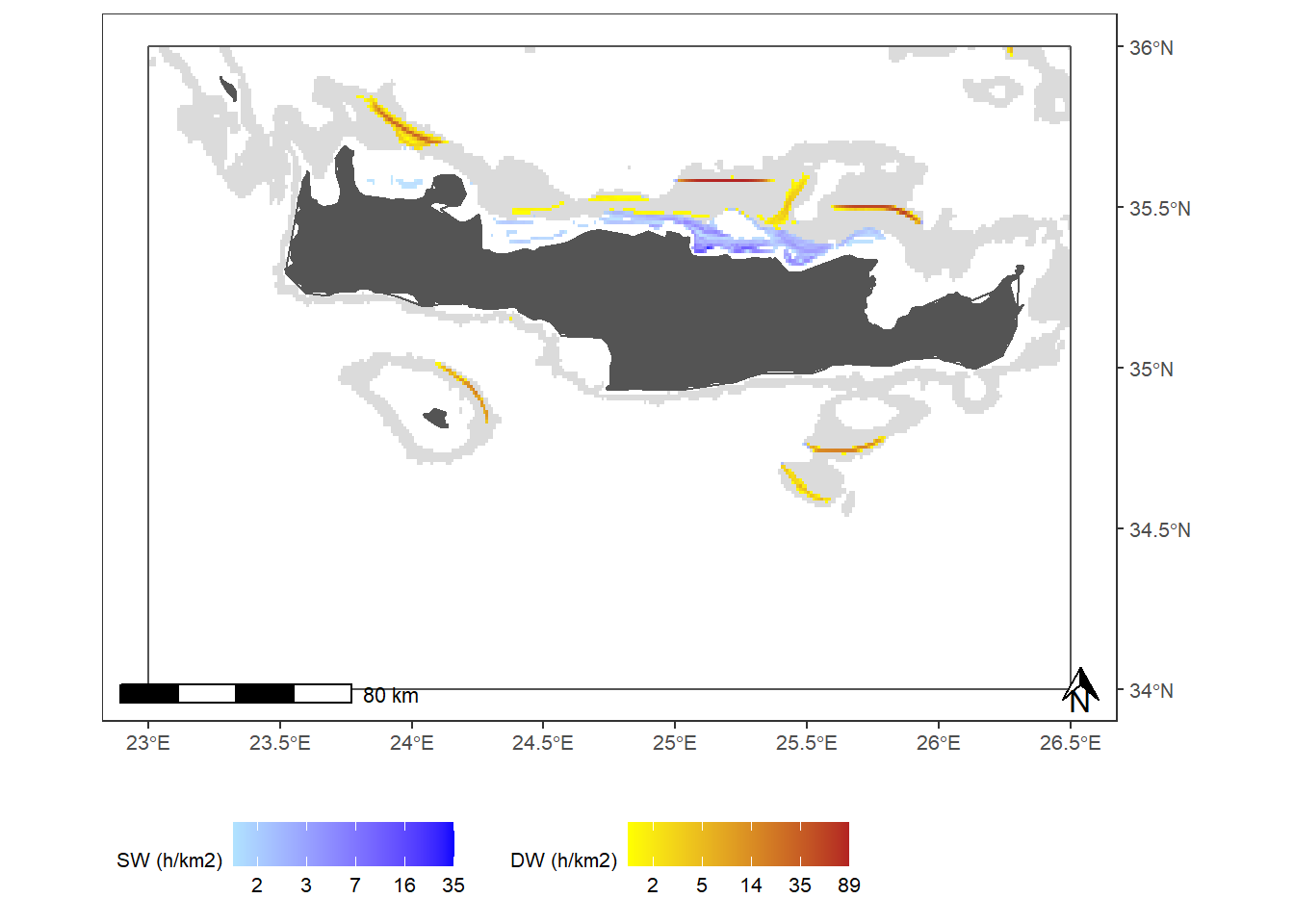

Fishing effort monthly time series

Step 1

The procedure is similar to what described in the Fishing effort map section, although here the values are calculate on monthly basis and summarized.

The monthly_effort dataset contains the cumulative monthly fishing hours by grid cell. In an additional line of code it is pasted a formatted information on the reference month.

monthly_effort=aggregate(list(nhours=fishing_data$f_hours), 
          by=list('year'= fishing_data$year, 'month'= fishing_data$month ,'DW'=fishing_data$DW), FUN=sum)

monthly_effort$temporal_ref=as.Date(paste(monthly_effort$year, monthly_effort$month, "01", sep = "-"))

year	month	nhours	temporal_ref
2016	1	0.6321288	2016-01-01
2018	1	0.0290744	2018-01-01
2017	2	0.0701169	2017-02-01
2018	2	344.5507970	2018-02-01
2016	3	0.3357668	2016-03-01
2017	3	0.5325699	2017-03-01

The vessel_by_month dataset contanins the monthly number of vessels fishing in the case study area, both for the DW and the SW batimetries. In an additional line of code it is pasted a formatted information on the reference month.

vessel_by_month=unique(fishing_data[,c('MMSI','month','year')])
vessel_by_month=aggregate(vessel_by_month$MMSI, 
                          by=list('year'=vessel_by_month$year , 'month'=vessel_by_month$month), FUN=length)
vessel_by_month$temporal_ref=as.Date(paste(vessel_by_month$year, vessel_by_month$month, "01", sep = "-"))

year	month	x	temporal_ref
2016	1	1	2016-01-01
2017	1	3	2017-01-01
2018	1	3	2018-01-01
2015	2	2	2015-02-01
2016	2	4	2016-02-01
2017	2	4	2017-02-01

Step 2

The monthly fishing hours and vessel statistics are calculated only for those months were fishing activity was actually observed. However we aim to consider in the plot also the months where no activity at all was observed. Therefore some formatting lines are needed.

index=data.frame(order=seq(1, 48, 1), 
           temporal_ref=seq(as.Date(paste("2015", "01", "01", sep = "-")),
                   as.Date(paste("2018", "12", "01", sep = "-")),"month"))

monthly_effort=merge(index, monthly_effort, by="temporal_ref", all.x = T)
monthly_effort[!is.na(monthly_effort$DW) & monthly_effort$DW==1,]$DW='DW'
monthly_effort[!is.na(monthly_effort$DW) & monthly_effort$DW==0,]$DW='SW'

vessel_by_month=merge(index, vessel_by_month, by="temporal_ref", all.x = T)

Plot

Specifications for the plot

Plots are standardized between figures using the settings loaded at the beginning of the script. In addition, labeling can be optimized to fit the data of each area.

plot_breaks=seq(min(monthly_effort$order),max(monthly_effort$order),3)
plot_labels=paste(substr(seq(min(monthly_effort$temporal_ref), 
                             max(monthly_effort$temporal_ref),"quarters"),1,4), 
                  month.abb[as.numeric(substr(seq(min(monthly_effort$temporal_ref),max(monthly_effort$temporal_ref),"quarters"),6,7))], sep="-")

Result

plot_effort_ts=defo_ts +
  geom_bar(data = monthly_effort, aes(x=order,y= nhours, fill = reorder(DW, desc(DW))), 
           stat = "identity", colour = 1, size=0.2) +
  scale_fill_manual(values = c("deepskyblue3", "tomato3")) + 
  xlab("")  + 
  scale_x_reverse(breaks=plot_breaks,labels=plot_labels)+
  guides(fill = guide_legend(title = "Fishing ground")) +
  ylab("Hours") +
  geom_line(data=vessel_by_month, aes(x=order, y = x*50), size = 0.7) +
  scale_y_continuous(sec.axis = sec_axis(~ . /50, name=expression(paste(""[""["No. DW trawlers"]], paste(bold(" __"))))), name=expression( ""[""["F hours"]])) ; plot_effort_ts

## Warning: Removed 5 rows containing missing values (position_stack).

## Warning: Removed 1 row(s) containing missing values (geom_path).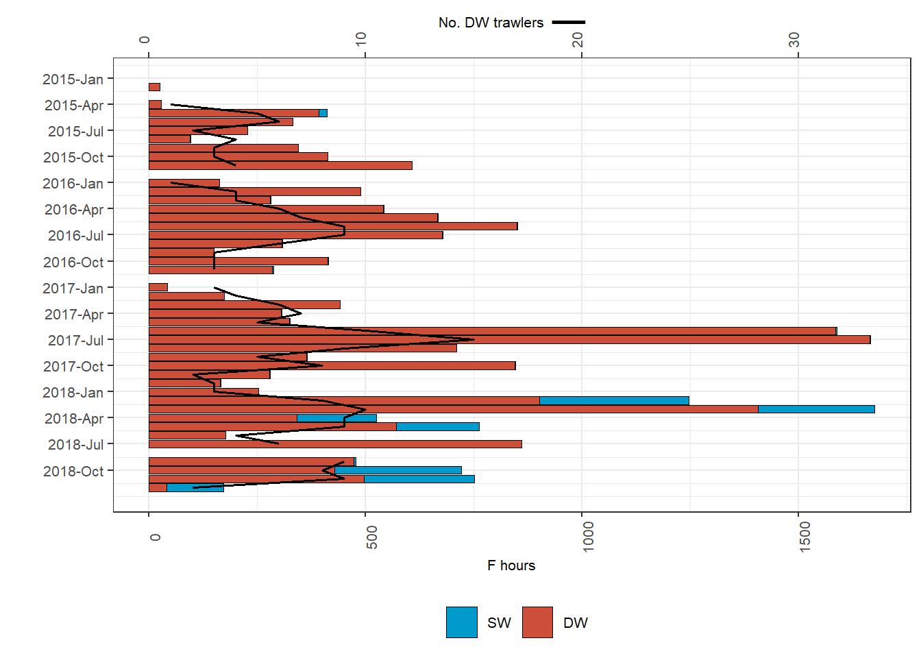

FishingIndicators

Before to start

Load data

fishing_data= read_csv("data/fishing_data.csv")


rm(vessel_selection)
# Shapefiles 
grid <- read_sf("maps/grid")

land=read_sf("maps/land")%>% 
  st_crop(., xmin=-10, xmax=43, ymin=20, ymax=48)

gsa=read_sf("maps/gsa")%>%
  dplyr::filter(SMU_CODE == '23' )

dep = read_sf("maps/depth_contours")%>%
  st_cast(., to = "POLYGON")%>%
  st_set_crs(st_crs(gsa))%>%
  st_buffer(0)%>%
  st_crop(gsa)

lims=c(st_bbox(gsa[c(1,3)], st_bbox(gsa[c(2,4)])))

text_size=8
plot_height=25
plot_width=18
source("R/supporting_code/plot_specifications.R")

Optional

In the following line there is the possibility to reduce the dataset by selecting only those vessels that fished in the DW strata at least once in a month.

vessel_selection=unique(fishing_data[fishing_data$DW==1,c('MMSI','month','year')]) # Create a monthly list of vessels fishing in the DW strata

fishing_data=merge(vessel_selection, fishing_data, by=c("MMSI", "year", "month"), all.x = T)

Indicator Map

Step 1

The indicator map is performed only for the DW stratum and over the entire reference period. As so, the first step requires to filter the input data to the reference batymetric stratum and to aggregate the fishing activity by grid cell over the 2015-208 period.

DWfishing_data=fishing_data[fishing_data$DW==1,]
DWfishing_data=aggregate(list('f_hours'=DWfishing_data$f_hours), 
                         by=list('G_ID'= DWfishing_data$G_ID), FUN=sum)

G_ID	f_hours
1867864	0.5300249
1868595	0.3755053
1869328	0.9126055
1870067	0.9154025
1870808	2.4478613
1870810	0.9643671

Step 2

The successive step relates to the calculation of the indicators. The dedicated functions are stored in a separate file for tidiness purpose and are shown below. The ind5 function serve to calculate the MSFD indicator D5, namely the extension of the fishing activity in a given area. It calculates the number of cells of the grid where fishing activity was observed over the reference period.

ind5=function(x){
  x = unique(x[,c('G_ID')])
  return(x)
}

The ind6 serve to calculate the MSFD indicator D6, namely the aggregation of the fishing activity in a given area. It calculates the number of cells of the grid containing the 90% of the cumulative distribution of the fishing activity over the refere

ind6=function(x){
  x = x[order(x$f_hours, decreasing = T),]
  x$cum = cumsum(x$f_hours)
  xthr = sum(x$f_hours, na.rm = T) * 0.9
  x=x[which(x$cum <= xthr),]
  return(x)
}

Both functions are applied to the data.

ind5_map=ind5(DWfishing_data)
ind6_map=ind6(DWfishing_data)

x
1867864
1868595
1869328
1870067
1870808
1870810

	G_ID	f_hours	cum
302	1981809	350.4092	350.4092
303	1982676	350.3049	700.7141
301	1980946	348.1182	1048.8323
312	1987953	346.2441	1395.0763
305	1983547	345.8874	1740.9637
311	1987063	344.1456	2085.1093

Step 3

Add the mean overall fishing intensity to the grid shapefile. For indicator 5 it is enough to filter the grid. For indicator 6 is done by using the merge function, using the G_ID column as primary key.

grid_ind5=grid[grid$G_ID%in%ind5_map,]
grid_ind6=merge(grid, ind6_map, by='G_ID', all.x=F)

G_ID	DW	GSA	EUNIScomb	grid_id	f_hours	cum	geometry
1873032	1	GSA23	A6.511	16217	42.63207	17813.37	POLYGON ((23.86001 35.81624…
1873776	1	GSA23	A6.511	16389	62.85778	16564.71	POLYGON ((23.87001 35.80624…
1874518	1	GSA23	A6.511	16562	96.66239	15052.40	POLYGON ((23.88001 35.79624…
1875256	1	GSA23	A6.511	16734	38.96086	18056.29	POLYGON ((23.89001 35.79624…
1875257	1	GSA23	A6.511	16735	91.00845	15520.13	POLYGON ((23.89001 35.78624…
1875994	1	GSA23	A6.511	16907	87.69846	15787.08	POLYGON ((23.90001 35.78624…

Plot

Specifications for the plot

Plots are standardized between figures using the settings loaded at the beginning of the script.

Result

plot_indicator_map = defo_map+
  geom_sf(data = grid_ind5, aes(fill = "orange"), colour = NA) +
  geom_sf(data = grid_ind6, aes(fill = "tomato3"), colour = NA) +
  scale_fill_identity(guide='legend',
                      breaks = c("orange", "tomato3"),
                      labels = c("Ext", "Agg"),
                      name='')+
  coord_sf(xlim=c(lims[[1]], lims[[3]]), ylim=c(lims[[2]], lims[[4]]) , label_axes = list(bottom = "E", right = "N"));plot_indicator_map

## Coordinate system already present. Adding new coordinate system, which will replace the existing one.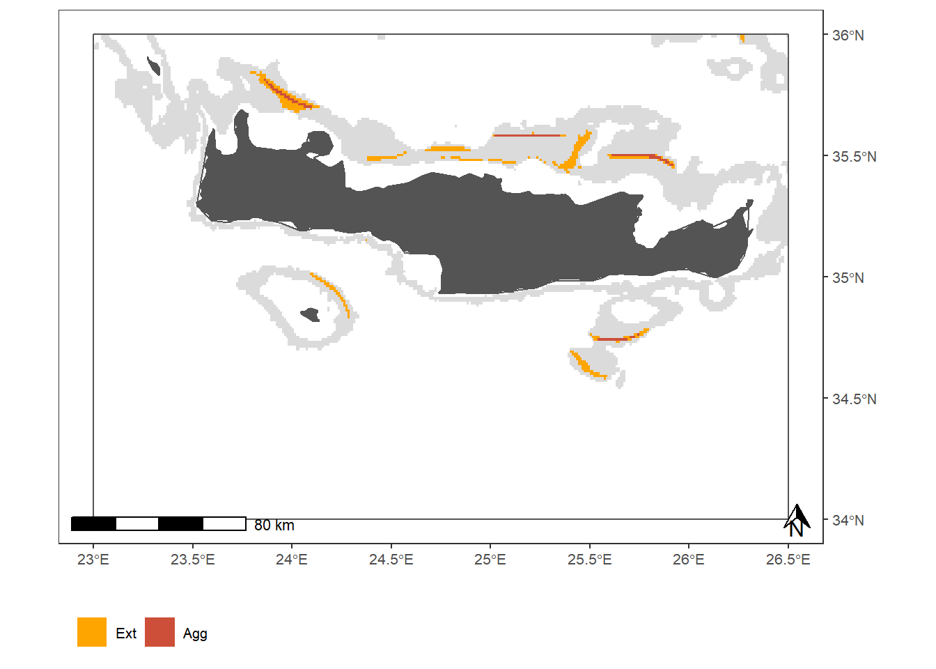

Indicators monthly time series

Step 1

The procedure is similar to what described in the Indicators map section, although the ind5 and ind6 functions here are applied on monthly basis.

First we define a temporal index, namely the month covering the period january 2015-december 2018

index=tibble(order=seq(1, 48, 1),
           temporal_ref=seq(as.Date(paste("2015", "01", "01", sep = "-")),
                   as.Date(paste("2018", "12", "01", sep = "-")),"month"))

order	temporal_ref
1	2015-01-01
2	2015-02-01
3	2015-03-01
4	2015-04-01
5	2015-05-01
6	2015-06-01

Then we build a for loop to iterate on each month contained in the temporal index. For each of the i timesteps, the data are filtered on the DW strata and the functions are applied. For each month we are interested in knowing the values assumed by the indicators, which in both cases are the number of cells falling in the indicator parameter. The ind_ts dataset serve to store all the monthly values, by adding the i value for each iteration over the time.

ind_ts=NULL
for (i in 1:nrow(index)){
  # Subset data
  idat=fishing_data[fishing_data$DW==1&
                      fishing_data$year==lubridate::year(index[i,]$temporal_ref)&
                      fishing_data$month==lubridate::month(index[i,]$temporal_ref),]
  if(nrow(idat)==0){
    next
    }else{
      i5=ind5(idat)
      idat=aggregate(list('f_hours'=idat$f_hours), by=list('G_ID'=idat$G_ID), FUN=sum)
      i6=ind6(idat)
      ind_ts = rbind(ind_ts, data.frame(temporal_ref=index[i,]$temporal_ref, dcf5=length(i5),dcf6=nrow(i6))) 
      rm(i5,i6, idat)
    }
}

After having calculated the indicator monthly values, we standardize them over the GSA extension.

grid_cells=data.frame(table(grid$DW, grid$GSA))
ind_ts$ncell_rbs=grid_cells[grid_cells$Var1==1,]$Freq
ind_ts$dcf5_ratio = round(ind_ts$dcf5/ind_ts$ncell_rbs,4)
ind_ts$dcf6_ratio = round(ind_ts$dcf6/ind_ts$ncell_rbs, 4) 
ind_ts$dcf_ratio = round((ind_ts$dcf6)/(ind_ts$dcf5),4)
ind_ts$temporal_ref=as.Date(ind_ts$temporal_ref)

temporal_ref	dcf5	dcf6	ncell_rbs	dcf5_ratio	dcf6_ratio	dcf_ratio
2015-02-01	59	38	7076	0.0083	0.0054	0.6441
2015-04-01	32	21	7076	0.0045	0.0030	0.6562
2015-05-01	110	52	7076	0.0155	0.0073	0.4727
2015-06-01	43	25	7076	0.0061	0.0035	0.5814
2015-07-01	58	24	7076	0.0082	0.0034	0.4138
2015-08-01	36	25	7076	0.0051	0.0035	0.6944

Step 2

ind_ts=merge(index, ind_ts, all.x = T)
ind_ts[is.na(ind_ts)]=0

The dataset is reshaped to fit into the plot specifications

ind_ts=reshape2:::melt(ind_ts[,c('temporal_ref','order', 'dcf5_ratio', 'dcf6_ratio')], id.var=1:2)
ind_ts$variable=factor(ifelse(ind_ts$variable == "dcf5_ratio", "Ext", "Agg"), levels = c("Ext", "Agg"))

temporal_ref	order	variable	value
2015-01-01	1	Ext	0.0000
2015-02-01	2	Ext	0.0083
2015-03-01	3	Ext	0.0000
2015-04-01	4	Ext	0.0045
2015-05-01	5	Ext	0.0155
2015-06-01	6	Ext	0.0061

Plot

Specifications for the plot

Plots are standardized between figures using the settings loaded at the beginning of the script. In addition, labeling can be optimized to fit the data of each area.

plot_breaks=seq(min(ind_ts$order),max(ind_ts$order),3)
plot_labels=paste(substr(seq(min(ind_ts$temporal_ref),max(ind_ts$temporal_ref),"quarters"),1,4),
                  month.abb[as.numeric(substr(seq(min(ind_ts$temporal_ref),max(ind_ts$temporal_ref),"quarters"),6,7))], sep="-")

Plot it!

plot_indicators_ts = defo_ts +
  geom_bar(data = ind_ts , aes(x=order, value, fill = variable), stat = "identity", colour = 1, na.rm = F, size=0.2) +
  scale_fill_manual(values = c("orange", "tomato3")) + 
  scale_x_reverse(breaks=plot_breaks, labels=plot_labels)+
  geom_hline( aes(yintercept = mean(ind_ts[is.na(ind_ts$value)==F & ind_ts$variable =="Ext", ]$value)))+
  geom_hline( aes(yintercept = mean(ind_ts[is.na(ind_ts$value)==F & ind_ts$variable =="Agg", ]$value)), linetype=2)+
  xlab("") +
  ylab("Proportion of DW")  + 
  guides(fill = guide_legend(title = "Indicator", size = 15), linetype=guide_legend())+
  scale_y_continuous(sec.axis = sec_axis(~ . /50,breaks=c(1),labels="", name=expression(paste(""[""["Ext "]],   bold("__"), ""[""["  Agg "]],bold("_ _") ))), name=expression(""[""["Proportion of DW"]]));plot_indicators_ts

## Warning in min(x): no non-missing arguments to min; returning Inf

## Warning in max(x): no non-missing arguments to max; returning -Inf

Workflow

Input data

Fishing data

Spatial layers

Processing

Pre processing

Before to start

Load spatial Data and set parameters

For loop sectioned

Step 1

Step 2

Step 3

Step 4 (Optional)

Results

FishingPattern

Before to start

Load data

Optional

Effort Map

Step 1

Step 2

Step 3

Plot

Specifications for the plot

Result

Fishing effort monthly time series

Step 1

Step 2

Plot

Specifications for the plot

Result

FishingIndicators

Before to start

Load data

Optional

Indicator Map

Step 1

Step 2

Step 3

Plot

Specifications for the plot

Result

Indicators monthly time series

Step 1

Step 2

Plot

Specifications for the plot

Plot it!